Introduction : Microsoft Excel is the go-to tool for working with data. There are probably a handful of people who haven’t used Excel, given its immense popularity. Excel is a widely used software application in industries today, built to generate reports and business insights. Excel supports several in-built applications that make it easier to use. 

One such feature that allows Excel to stand out is - Excel sheet formulas. Here, we will look into the top 25 Excel formulas that one must know while working on Excel. The topics that we will be covering  in this article are as follows:

What is Excel Formula? 

In Microsoft Excel, a formula is an expression that operates on values in a range of cells. These formulas return a result, even when it is an error. Excel formulas enable you to perform calculations such as addition, subtraction, multiplication, and division. In addition to these, you can find out averages and calculate percentages in excel for a range of cells, manipulate date and time values, and do a lot more.

Excel formulas are used to do mathematical calculations. The users can use the formulas to do complex calculations. There are two ways to do the calculations in the sheet one is using the formulas or the functions. 

Formulas in Excel: An Overview

1. Choose a cell.
2. To enter an equal sign, click the cell and type =.
3. Enter the address of a cell in the selected cell or select a cell from the list.
4. You need to enter an operator.
5. Enter the address of the next cell in the selected cell.
6. Press Enter.

The benefits of learning Excel Formulas 

For those who are wondering about learning Excel formulas and spending time on it worth a shot? In a recent survey conducted more than 90% of employees responded that Excel formulas are vital to their job. 

Top 5 Reasons to learn Excel Formulas 

1. Of course, it makes your job a lot easier 
2. Enhancing your skill sets – is always an added advantage 
3. Better at organizing the data
4. Making you a valuable employee for the company 
5. Increases the efficiency and productivity 

The most widely used function in excel, allows you to find the total of a particular column or the selected range of cell values. Mathematically it is calculated to find the total added value (addition) 

1. SUM function 

Formula =SUM(num1,num2,…)

Example

To find the total the amount 

Under the Amount column for Fruit (cell B6), enter =SUM(B2:B5), or type =SUM(, then select that range with the mouse, and press Enter. This will sum the values in cells B2, B3, B4, and B5. Your answer should be 170.

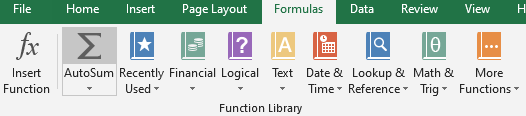
AUTOSUM 

Now let’s try AutoSum. Select the yellow cell under the column for the Amount  (cell B6), then go to Formulas > AutoSum > select SUM. You’ll see Excel automatically enter the formula for you. Press Enter to confirm it. The AutoSum feature has all of the most common functions.

A keyboard shortcut. Select cell B6, then press Alt and =  then, Enter. This automatically enters SUM for you.

2. AVERAGE function

The AVERAGE function is used to get the average of numbers in a range of cells. 

Formula =AVERAGE(num1,num2,..)

Select cell B6, and enter an AVERAGE function by typing **=AVERAGE(B2:B5). **

3. MIN and MAX functions

The MIN function is used to get the smallest number in a range of cells.

The MAX function is used to get the largest number in a range of cells.

4. COUNT 

The COUNT function allows you to find the total count of entries in the cells that contain numbers. 

Formula =COUNT(value1,value2,..)

Example: To count the number of cells or array of numbers in B cell, select B14 and enter =COUNT(B1:B13). You can see the count of the cell which has a number alone taken. 

If you need to count the cells, which contain all the values like numbers, text, and any other data format, you can use COUNTA() this does not include the blank cells 

COUNTBLANK() to count the cells that are blank 

5. IF statements

IF statements let you make logical comparisons between conditions. It generally says that if one condition is true do something, otherwise do something else. The formulas, return text, values, or even more calculations

Formula =IF(Logical_test,[value_if_true],[value_if_false

For Example

In cell B2 enter =IF(A2=”Apple”,TRUE,FALSE). The correct answer is TRUE.

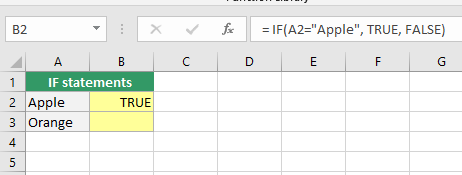
Apply the same formula to B3. The answer here should be FALSE, because orange is not an apple.

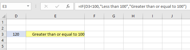
Try another example by looking at the formula in cell E3. We got you started with =IF(D3<100,”Less than 100″,”Greater than or equal to 100″). What happens if you enter a number greater than or equal to 100 in cell D3?

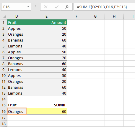
6. Conditional Functions – SUMIF 

Conditional functions let you sum, average, count, or get the min or max of a range based on a given condition, or criteria you specify. Such as, out of all the fruits on the list, how many are apples? Or, how many oranges are the Florida type?

Formula =SUMIF(range,criteria,[sum_range])

Example 

SUMIF lets you sum in one range based on specific criteria you look for in another range, like how many Oranges you have. Select cell E16 and type =SUMIF(D2:D13,D16,E2:E13). 

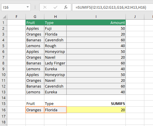
SUMIFS is the same as SUMIF, but it lets you use multiple criteria. 

Formula =SUMIFS(sum_range,criteria_range1,criteria1,criteria_range2…..)

So in this example, you can look for Fruit and Type, instead of just by Fruit. Select cell I16 and type =SUMIFS(I2:I13,G2:G13,I16,H2:H13,H16)

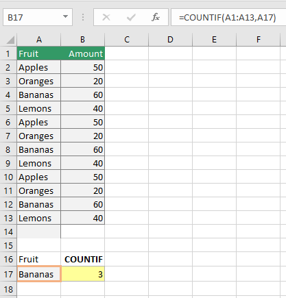
7. COUNTIF 

The function COUNTIF is used when you are required to count cells with specified criteria.

Formula =COUNTIF(range,criteria)

Example:  To count the cell which contains a specific fruit name like Banana, you need to select cell B17 and enter =COUNTIF(A1:A13,A17)

COUNTIFS is the same as SUMIF, but it lets you use multiple criteria. 

Formula =COUNTIFS(criteria_range1,criteria1,..)

So in this example, you can look for Fruit and Type, instead of just by Fruit. Select cell F17 and type =COUNTIFS(D2:D13,D17,E2:E13,E17). 

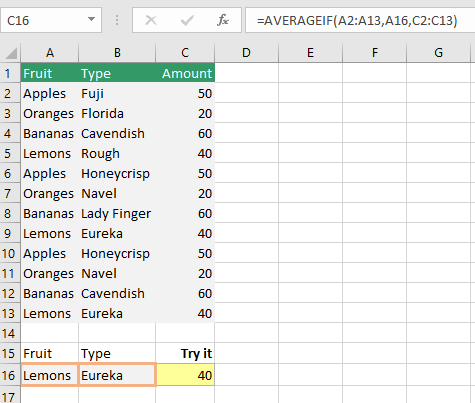
8. AVERAGEIF

The AVERAGEIF in the excel returns you the average value in a range with the specified criteria. The specified criteria can be numbers, strings, or references. 

Formula =AVERAGEIF( (range, criteria, [average_range])

Example: The average price of the lemons is retuned by entering =AVERAGEIF((A2:A13,A16,C2:C13)

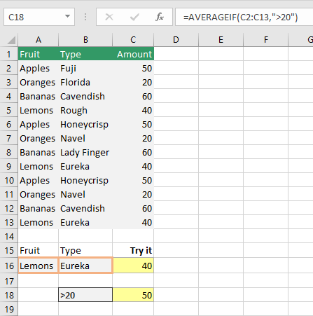
 In the second example, we have got the average price of Fruits which is more than the cost of 20 by entering =AVERAGEIF(C2:C13,”>20″)

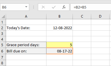
9. TODAY

TODAY function gives you Today’s date. These are live functions, so whenever you open the workbook, it will have an updated date. Enter =TODAY() in the cell. 

Add Dates – Let’s say you want to know the bill due date, or when you need to return a book. You can add days to a date to find out. In cell B5, enter a random number of days. In cell B6, we added =B2+B5 to calculate the due date today.

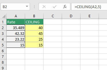
 10. Ceiling and Floor function

The Excel CEILING function rounds up to the nearest given multiple numbers. Use CEILING(number) always to ROUND UP the value 

Example 

In the below sheet we have used CEILING to round up the rate (number) to the multiple of 5 (significance). In cell B2 enter =CEILING(A2,5)

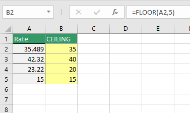
*FLOOR *

Excel FLOOR function is the same but rounds down to the nearest given multiples. The FLOOR() is always used to ROUND DOWN the value 

Example 

In the below sheet we have used FLOOR to round down the rate (number) to the nearest multiple of 5 (significance). In cell B2 enter =FLOOR(A2,5)

11. VLOOKUP

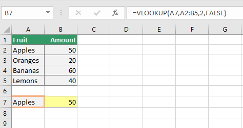
VLOOKUP is the most famous and widely used function, it is the Vertical Lookup in Excel. As the name suggests it is the Excel function that helps to look up specified values vertically. It helps you look up for value in the left column and then returns information in another column to the right if it finds a match. 

Formula =VLOOKUP(lookup_value,tabe_array,col_index_num,[range_lookup]

Example 

In cell B7, enter =VLOOKUP(A7,A2:B5,2,FALSE). The correct answer for Apples is 50. VLOOKUP looked for Apples, found them, then went over one column to the right, and returned the amount.

 VLOOKUP Formula structured as 

1. A7 – What do you want to look for?
2. A2:B5 – Where do you want to look for it?
3. 2 – If you find it, how many columns to the right do you want to get a value?
4. FALSE – Do you want an exact, or 
5. TRUE –  in case of an approximate match?

If VLOOKUP returns an error (#N/A) then it means that the searched value does not exist in the sheet. 

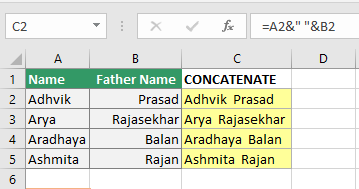
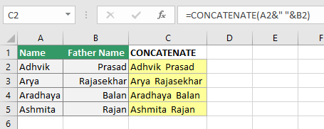
12. CONCATENATE

The word CONCATENATE means to combine. This Excel function simply means to combine different texts from different cells into one cell. The user can do this in two ways either using the build Excel function or the formula.

Formula =CONCATENATE(TEXT1,TEXT2,..)

Example 

=A1&B1 gives the same results as** **

=CONCATENATE(A1,B1)

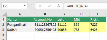
13. LEFT, MID, RIGHT

LEFT function –  To extract the given number of characters from the left of the text 

Formula – =LEFT(text,num_charc)

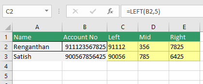
 MID function – To extract from the middle of the characters in the text, with the given starting position and the number of characters 

Formula =MID(text,start_num,num_charc)

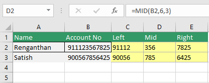
 RIGHT function – To extract the given number of characters from the right of the text 

Formula =RIGHT(text,num_charc)

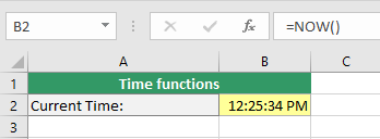
14. Time functions – NOW

Excel can give you the current time, based on your computer’s regional settings. You can also add and subtract times. For instance, you might need to keep track of how many hours an employee worked each week, and calculate their pay and overtime.

enter =NOW(), which will give the current time, and will update each time Excel calculates. If you need to change the Time format, you can go to Ctrl+1 > Number > Time > Select the format you want.

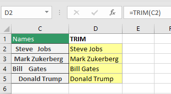
15. TRIM

When you receive a worksheet with irregular spaces and the user wants to organize it, then excel has a great function TRIM that cuts out the unwanted spaces in the cell. 

Enter =TRIM(text) to remove the unwanted spaces in the cell

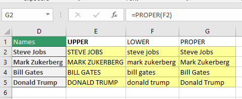
16. UPPER, LOWER, PROPER

UPPER function – To convert the texts to uppercase. =UPPER()

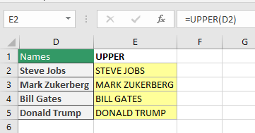
 LOWER function – To convert the texts to lowercase. =LOWER()

PROPER function – To convert all the improper texts into the correct format 

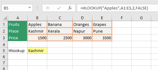
17. HLOOKUP

HLOOKUP does the exact same function as VLOOKUP but instead searches for a certain value in the rows in the excel sheet, whereas VLOOKUP searches the column.

Example: Enter =HLOOKUP(lookup_value, table_array, row_index_num, [range_lookup])

1. Lookup value – Apples 

2. Table array – the table in which the data is looked up 

3. Row index num – the row number in the table array from which the matching value is returned 

4. Range lookup – Exact match or approximate match 

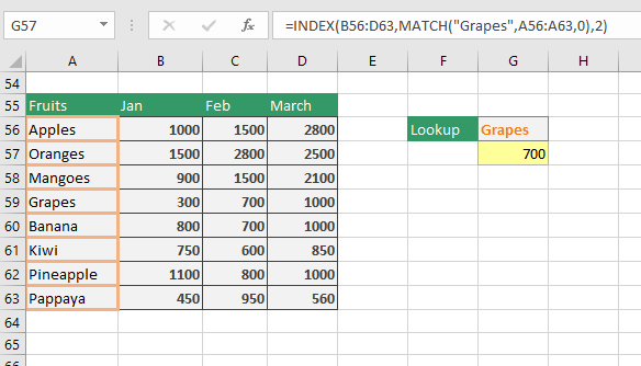
   18. INDEX and MATCH

INDEX and MATCH is the most popular tool in Excel for carrying out more advanced lookups. This is because INDEX and MATCH are extremely flexible – you can do horizontal and vertical lookups, 2-way lookups, left lookups, case-sensitive lookups, and even lookups based on multiple criteria. If you want to enhance your Excel skills, INDEX and MATCH are musts.

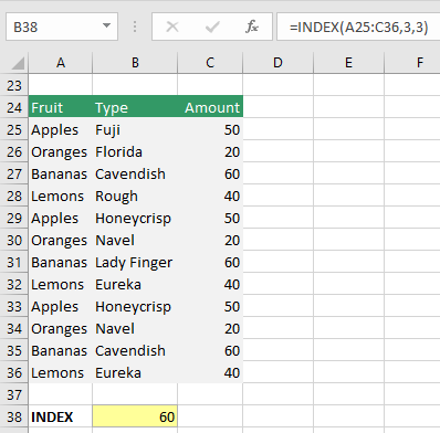
The Excel INDEX function returns the value of a given location in a range or array. You can use INDEX to retrieve individual values, or entire rows and columns. However, the MATCH function is often used together with INDEX to provide row and column numbers.

Formula  =INDEX (array, row_num, [col_num])

For example – in the below list to retrieve data from the required row and column enter =INDEX(A25:C36,3,3)

*MATCH*

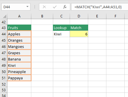
This excel function retrieves the location of the specified value from the row, column, and table in the spreadsheet. 

Formula – =MATCH (lookup_value, lookup_array, [match_type])

In the below example we are looking for the position of Kiwi, so enter =MATCH(“Kiwi”,A44:A51,0)

 Note: Match type 

1. 1 – return the approximate lookup value / Less than value

2. 0 – Exact lookup value 

3. -1 –  More than the lookup value 

   

 To sum up, the INDEX returns the value of the given position whereas MATCH returns the position of the lookup value.

The user can combine both INDEX and MATCH functions, 

To lookup the value of Grapes in the month of Feb, enter =INDEX(B56:D63,MATCH(“Grapes”,A56:A63,0),2)

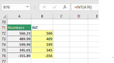
 19. INT

In Excel, the INT function is used to remove the decimal from the numbers. This just eliminates the decimals and doesn’t round up or round down to the nearest value. But in case the cell has a negative value then INT acts different by rounding up/ down 

=INT(Num)

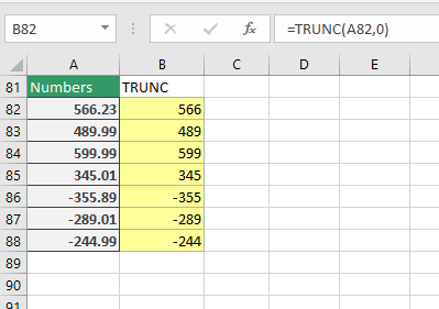
20. TRUNC

The TRUNC function in Excel is the same as INT but this removes the decimal be it any value entered in the cell.

Formula =TRUNC(number,[num_digits])

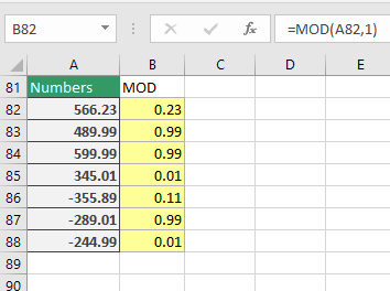
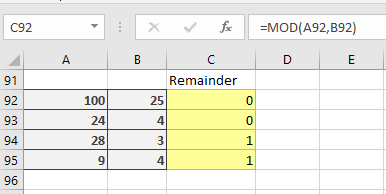
21. MOD

This Excel function is used in two ways. First, used when you want to extract the decimal part of the value. Second to get the remainder after the division 

Formula =MOD(number,divisior)

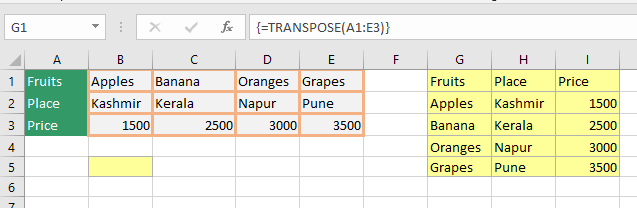
22. TRANSPOSE

This Excel function can be used to transpose your data from Horizontal to vertical or vice versa. 

As it is an array formula user needs to CTRL+SHIFT+ENTER the formula to get the results. 

In the below sheet, the horizontal data has been converted vertically using =TRANSPOSE(array)

1. Select the exact space to convert the value 
2. Enter the formula 
3. Press CTRL+SHIFT+ENTER

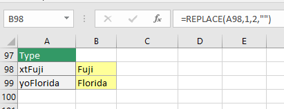
23. REPLACE

This Excel function is used when the user wants to replace a certain specified text or number with a different value or to remove it. The user needs to give the exact location and the new value to get the result 

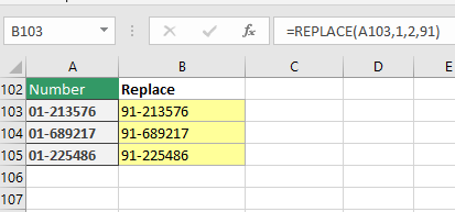
Formula: =REPLACE(old_text, start_num, num_chars, new_text)

We have two examples- To Remove certain text enter =REPLACE(A98,1,2,””)

 To replace a value enter =REPLACE(A103,1,2,91)

24. RAND and RANDBETWEEN

The RAND excel function retrieves a random number every time an excel sheet is opened or calculated. 

=RAND() returns a value >= to 0 and < 1

=RAND()*100 returns a number >=0 less than 100

=INT(RAND()*100) returns a random whole number >=0 and less than 100

=RANDBETWEEN(top, bottom) returns a random number within the specified limit 

25. ROW, ROWS, COLUMN, COLUMNS

1. ROW – To get the ROW number of any cell
2. ROWS – To get the count of the selected array of ROWS
3. COLUMN – To get the COLUMN number of the given cell
4. COLUMNS – To get the count of the selected array of COLUMNS

In today’s business world, there is a large use of Microsoft Excel. And it is necessary for everyone to learn the basic formula of Excel, which benefits you in so many ways. There is high demand for Excel skill sets as it is required by vast industries and companies.

If you want to enhance your skills with Advanced Excel knowledge you may check out the course offered.

Excel has been there and will always be there for various purposes and the application has various features and functions that helps you to simplify the work. No matter what field you are in, learning the basics of MS Excel will help you in many ways. Those who are keen to know more about the feature and looking to enhance their skills can enroll in the courses offered.